Fastai BW data augmentation

Experimenting with Fastai and BW data augmentation.

Runpod setup

# setting up pod and pip install uhina
# accessing a pod terminal

# 1. To get access to the pod ip adress: runpodctl get pod -a
# 2. ssh into the pod: ssh root@<ip-address> -p 58871 -i ~/.ssh/id_ed25519


# runpodctl send uhina 

# git clone https://github.com/franckalbinet/uhina.git
# pip install uhina
# runpodctl send im-bw 
# runpodctl send ossl-tfm.csv

Loading data

import pandas as pd
from pathlib import Path
import fastcore.all as fc

from fastai.data.all import *
from fastai.vision.all import *
from multiprocessing import cpu_count
from uhina.augment import Quantize

import warnings
warnings.filterwarnings('ignore')

ossl_source = '../../_data/ossl-tfm/im-targets-lut.csv'
df = pd.read_csv(ossl_source); df.head()

	fname	kex
0	3998362dd2659e2252cd7f38b43c9b1f.png	0.182895
1	2bab4dbbac073b8648475ad50d40eb95.png	0.082741
2	29213d2193232be8867d85dec463ec00.png	0.089915
3	8b1ee9146c026faee20a40df86736864.png	0.135030
4	6e8e9d1105e7da7055555cb5d310df5f.png	0.270421

df['kex'].min(), df['kex'].max()

(0.0, 3.6521352871126975)

from sklearn.model_selection import train_test_split
df_train, df_valid = train_test_split(df, test_size=0.1, random_state=41)
idx_train, idx_valid = df_train.index, df_valid.index
len(idx_train), len(idx_valid)

(51906, 5768)

class OrderedQuantize(Quantize):
    order = 0  # Apply first

class OrderedRatioResize(RatioResize):
    order = 1  # Apply second

def splitter(items): return [idx_train, idx_valid]
    
ossl = DataBlock(
    blocks=(ImageBlock, RegressionBlock),
    get_x=ColReader(0, pref='../../_data/ossl-tfm/im/'),
    get_y=ColReader(1),
    splitter=splitter,
    item_tfms=[OrderedQuantize(n_valid=len(idx_valid))],
    batch_tfms=[
        OrderedRatioResize(224),
        Normalize.from_stats(*imagenet_stats)
    ]
)

#def splitter(items): return [idx_train, idx_valid]

#ossl = DataBlock(blocks=(ImageBlock, RegressionBlock),
#                get_x=ColReader(0, pref='../../_data/ossl-tfm/im/'),
#                get_y=ColReader(1),
#                # batch_tfms=Normalize.from_stats(*imagenet_stats),
#                batch_tfms=[RatioResize(224)],
#                item_tfms=[Quantize(n_valid=len(idx_valid))],
#                # splitter=RandomSplitter(valid_pct=0.1, seed=41)
#                splitter=splitter
#    batch_tfms=aug_transforms()
#)

# ossl.summary(df)

dls = ossl.dataloaders(df)

dls.show_batch(nrows=6, ncols=2, figsize=(12, 13))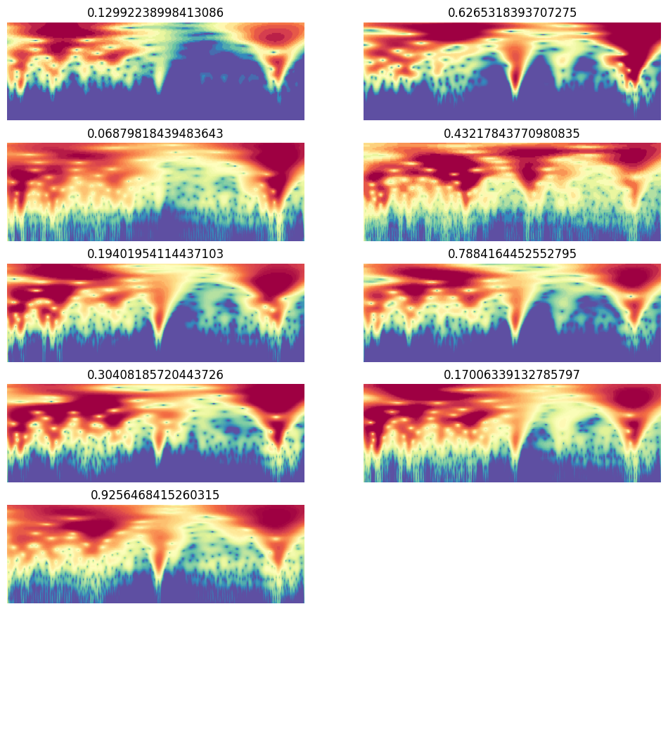

learn = vision_learner(dls, resnet18, pretrained=True, metrics=R2Score()).to_fp16()

learn.freeze()

learn.lr_find()

SuggestedLRs(valley=0.0010000000474974513)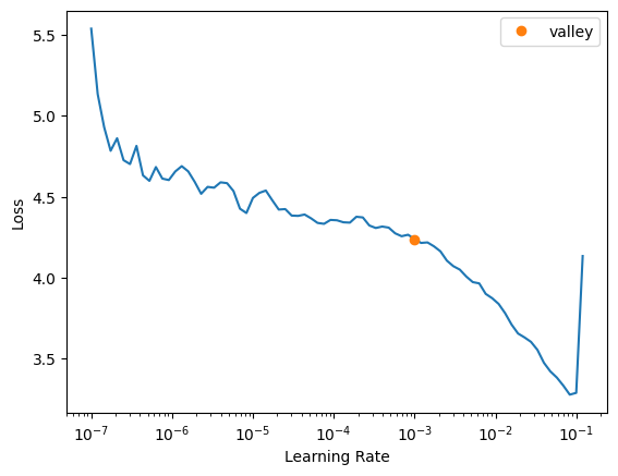

#learn.summary()

Sequential (Input shape: 64 x 3 x 221 x 669)
============================================================================
Layer (type)         Output Shape         Param #    Trainable 
============================================================================
                     64 x 64 x 111 x 335 
Conv2d                                    9408       True      
BatchNorm2d                               128        True      
ReLU                                                           
____________________________________________________________________________
                     64 x 64 x 56 x 168  
MaxPool2d                                                      
Conv2d                                    36864      True      
BatchNorm2d                               128        True      
ReLU                                                           
Conv2d                                    36864      True      
BatchNorm2d                               128        True      
Conv2d                                    36864      True      
BatchNorm2d                               128        True      
ReLU                                                           
Conv2d                                    36864      True      
BatchNorm2d                               128        True      
____________________________________________________________________________
                     64 x 128 x 28 x 84  
Conv2d                                    73728      True      
BatchNorm2d                               256        True      
ReLU                                                           
Conv2d                                    147456     True      
BatchNorm2d                               256        True      
Conv2d                                    8192       True      
BatchNorm2d                               256        True      
Conv2d                                    147456     True      
BatchNorm2d                               256        True      
ReLU                                                           
Conv2d                                    147456     True      
BatchNorm2d                               256        True      
____________________________________________________________________________
                     64 x 256 x 14 x 42  
Conv2d                                    294912     True      
BatchNorm2d                               512        True      
ReLU                                                           
Conv2d                                    589824     True      
BatchNorm2d                               512        True      
Conv2d                                    32768      True      
BatchNorm2d                               512        True      
Conv2d                                    589824     True      
BatchNorm2d                               512        True      
ReLU                                                           
Conv2d                                    589824     True      
BatchNorm2d                               512        True      
____________________________________________________________________________
                     64 x 512 x 7 x 21   
Conv2d                                    1179648    True      
BatchNorm2d                               1024       True      
ReLU                                                           
Conv2d                                    2359296    True      
BatchNorm2d                               1024       True      
Conv2d                                    131072     True      
BatchNorm2d                               1024       True      
Conv2d                                    2359296    True      
BatchNorm2d                               1024       True      
ReLU                                                           
Conv2d                                    2359296    True      
BatchNorm2d                               1024       True      
____________________________________________________________________________
                     64 x 512 x 1 x 1    
AdaptiveAvgPool2d                                              
AdaptiveMaxPool2d                                              
____________________________________________________________________________
                     64 x 1024           
Flatten                                                        
BatchNorm1d                               2048       True      
Dropout                                                        
____________________________________________________________________________
                     64 x 512            
Linear                                    524288     True      
ReLU                                                           
BatchNorm1d                               1024       True      
Dropout                                                        
____________________________________________________________________________
                     64 x 1              
Linear                                    512        True      
____________________________________________________________________________

Total params: 11,704,384
Total trainable params: 11,704,384
Total non-trainable params: 0

Optimizer used: <function Adam>
Loss function: FlattenedLoss of MSELoss()

Model unfrozen

Callbacks:
  - TrainEvalCallback
  - CastToTensor
  - MixedPrecision
  - Recorder
  - ProgressCallback

learn.fit_one_cycle(30, 1.5e-3)

epoch	train_loss	valid_loss	r2_score	time
0	1.644630	0.300183	-1.107600	03:27
1	0.330966	0.122813	0.137722	03:24
2	0.111735	0.096092	0.325332	03:24
3	0.090042	0.080140	0.437336	03:23
4	0.086476	0.076293	0.464347	03:24
5	0.079303	0.067029	0.529383	03:26
6	0.079823	0.077337	0.457015	03:21
7	0.071064	0.063280	0.555711	03:26
8	0.063395	0.049661	0.651327	03:25
9	0.064540	0.050022	0.648795	03:20
10	0.056607	0.048462	0.659747	03:22
11	0.053760	0.053292	0.625835	03:23
12	0.056411	0.048289	0.660963	03:20
13	0.049446	0.046147	0.676001	03:26
14	0.047927	0.041901	0.705815	03:26
15	0.046742	0.044546	0.687241	03:28
16	0.049120	0.041590	0.707998	03:18
17	0.043476	0.039859	0.720151	03:27
18	0.046412	0.038752	0.727923	03:22
19	0.044368	0.040569	0.715167	03:18
20	0.040819	0.037822	0.734452	03:24
21	0.043126	0.036971	0.740424	03:22
22	0.042248	0.036392	0.744487	03:16
23	0.041793	0.036009	0.747177	03:22
24	0.039837	0.035846	0.748324	03:22
25	0.039785	0.035595	0.750088	03:27
26	0.040293	0.035616	0.749942	03:29
27	0.037746	0.035546	0.750431	03:25
28	0.038235	0.036200	0.745835	03:21
29	0.038197	0.035067	0.753795	03:25

learn.unfreeze()

learn.lr_find()

SuggestedLRs(valley=1.2022644114040304e-05)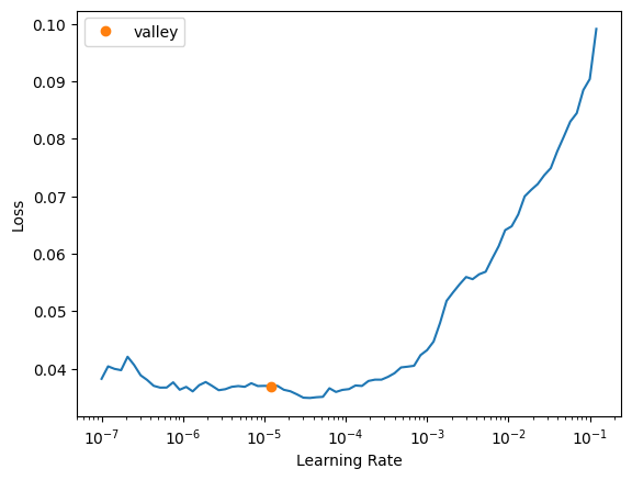

learn.fit_one_cycle(10, slice(1e-5, 1e-4))

epoch	train_loss	valid_loss	r2_score	time
0	0.041027	0.036716	0.742214	03:24
1	0.043233	0.038476	0.729859	03:25
2	0.040227	0.036917	0.740801	03:27
3	0.037694	0.032176	0.774093	03:34
4	0.033340	0.032090	0.774694	03:20
5	0.029570	0.030667	0.784687	03:22
6	0.027940	0.028028	0.803215	03:24
7	0.028264	0.027417	0.807507	03:23
8	0.025013	0.026760	0.812116	03:17
9	0.024846	0.026566	0.813480	03:22

Evaluation

val_preds, val_targets = learn.get_preds(dl=dls.valid)

r2_score(val_preds, val_targets)

0.7777369823359973

val_preds_tta, val_targets_tta = learn.tta(dl=dls.valid, n=10)

from sklearn.metrics import r2_score
r2_score(val_preds_tta, val_targets_tta)

0.7900635997635996

# EXAMPLE of TTA on single item
# from fastai.vision.all import *

# # Define your TTA transforms
# tta_tfms = [
#     RandomResizedCrop(224, min_scale=0.5),
#     Flip(),
#     Rotate(degrees=(-15, 15)),
#     Brightness(max_lighting=0.2),
#     Contrast(max_lighting=0.2)
# ]

# # Create a pipeline of TTA transformations
# tta_pipeline = Pipeline(tta_tfms)

# # Load your model
# learn = load_learner('path/to/your/model.pkl')

# # Define the input data (e.g., an image)
# input_data = PILImage.create('path/to/your/image.jpg')

# # Apply TTA transforms to the input data and make predictions
# predictions = []
# for _ in range(5):  # Apply 5 different augmentations
#     augmented_data = tta_pipeline(input_data)
#     prediction = learn.predict(augmented_data)
#     predictions.append(prediction)

# # Average the predictions
# average_prediction = sum(predictions) / len(predictions)

# print(average_prediction)

# Assuming you have a new CSV file for your test data
# test_source = '../../_data/ossl-tfm/ossl-tfm-test.csv'
# test_df = pd.read_csv(test_source)

# # Create a new DataLoader for the test data
# test_dl = learn.dls.test_dl(test_df)

# # Get predictions on the test set
# test_preds, test_targets = learn.get_preds(dl=test_dl)

# # Now you can use test_preds and test_targets for further analysis

# Convert predictions and targets to numpy arrays
def assess_model(val_preds, val_targets):
    val_preds = val_preds.numpy().flatten()
    val_targets = val_targets.numpy()

    # Create a DataFrame with the results
    results_df = pd.DataFrame({
        'Predicted': val_preds,
        'Actual': val_targets
    })

    # Display the first few rows of the results
    print(results_df.head())

    # Calculate and print the R2 score
    from sklearn.metrics import r2_score
    r2 = r2_score(val_targets, val_preds)
    print(f"R2 Score on validation set: {r2:.4f}")

assess_model(val_preds, val_targets)

   Predicted    Actual
0   0.312483  0.000000
1   0.126990  0.184960
2   0.365726  0.194201
3   0.239089  0.262364
4   0.402980  0.355799
R2 Score on validation set: 0.8325

assess_model(val_preds_tta, val_targets_tta)

   Predicted    Actual
0   0.246857  0.000000
1   0.148590  0.184960
2   0.371643  0.194201
3   0.226535  0.262364
4   0.407333  0.355799
R2 Score on validation set: 0.8378

val_preds_np = val_preds
val_targets_np = val_targets

# Apply the transformation: exp(y) - 1
val_preds_transformed = np.exp(val_preds_np) - 1
val_targets_transformed = np.exp(val_targets_np) - 1

# Create a DataFrame with the results
results_df = pd.DataFrame({
    'Predicted': val_preds_transformed,
    'Actual': val_targets_transformed
})

# Display the first few rows of the results
print(results_df.head())

# Calculate and print the R2 score
from sklearn.metrics import r2_score
r2 = r2_score(val_targets_transformed, val_preds_transformed)
print(f"R2 Score on validation set (after transformation): {r2:.4f}")

# Calculate and print the MAPE, handling zero values
def mean_absolute_percentage_error(y_true, y_pred):
    non_zero = (y_true != 0)
    return np.mean(np.abs((y_true[non_zero] - y_pred[non_zero]) / y_true[non_zero])) * 100

mape = mean_absolute_percentage_error(val_targets_transformed, val_preds_transformed)
print(f"Mean Absolute Percentage Error (MAPE) on validation set: {mape:.2f}%")

# Calculate and print the MAE as an alternative metric
from sklearn.metrics import mean_absolute_error
mae = mean_absolute_error(val_targets_transformed, val_preds_transformed)
print(f"Mean Absolute Error (MAE) on validation set: {mae:.4f}")

   Predicted   Actual
0   0.366814  0.00000
1   0.135405  0.20317
2   0.441560  0.21434
3   0.270092  0.30000
4   0.496277  0.42732
R2 Score on validation set (after transformation): 0.6936
Mean Absolute Percentage Error (MAPE) on validation set: 50.72%
Mean Absolute Error (MAE) on validation set: 0.1956

plt.figure(figsize=(6, 6))

# Use logarithmic bins for the colormap
h = plt.hexbin(val_targets, val_preds, gridsize=65, 
               bins='log', cmap='Spectral_r', mincnt=1,
               alpha=0.9)

# Get the actual min and max counts from the hexbin data
counts = h.get_array()
min_count = counts[counts > 0].min()  # Minimum non-zero count
max_count = counts.max()

# Create a logarithmic colorbar
cb = plt.colorbar(h, label='Count in bin', shrink=0.73)
tick_locations = np.logspace(np.log10(min_count), np.log10(max_count), 5)
cb.set_ticks(tick_locations)
cb.set_ticklabels([f'{int(x)}' for x in tick_locations])

# Add the diagonal line
min_val = min(val_targets.min(), val_preds.min())
max_val = max(val_targets.max(), val_preds.max())
plt.plot([min_val, max_val], [min_val, max_val], 'k--', lw=1)

# Set labels and title
plt.xlabel('Actual Values')
plt.ylabel('Predicted Values')
plt.title('Predicted vs Actual Values (Hexbin with Log Scale)')

# Add grid lines
plt.grid(True, linestyle='--', alpha=0.65)

# Set the same limits for both axes
plt.xlim(min_val, max_val)
plt.ylim(min_val, max_val)

# Make the plot square
plt.gca().set_aspect('equal', adjustable='box')

plt.tight_layout()
plt.show()

# Print the range of counts in the hexbins
print(f"Min non-zero count in hexbins: {min_count}")
print(f"Max count in hexbins: {max_count}")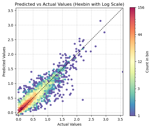

Min non-zero count in hexbins: 1.0
Max count in hexbins: 157.0

path_model = Path('./models')
learn.export(path_model / 'frozen-epoch-30-lr-1.5e-3-then-unfrozen-epoch-10-lr-1-e-4-12102024.pkl')

Inference

ossl_source = Path('../../_data/ossl-tfm/img')
learn.predict(ossl_source / '0a0a0c647671fd3030cc13ba5432eb88.png')

((0.5229991674423218,), tensor([0.5230]), tensor([0.5230]))

df[df['fname'] == '0a0a0c647671fd3030cc13ba5432eb88.png']

	fname	kex
28867	0a0a0c647671fd3030cc13ba5432eb88.png	0.525379

np.exp(3) - 1

19.085536923187668

Experiments:

Color scale: viridis | Discretization: percentiles = [i for i in range(60, 100)]

Model	Image Size	Learning Rate	Epochs	R2 Score	Time per Epoch	Finetuning	with axis ticks
ResNet-18	100	1e-3	10	0.648	05:12	No	Yes
ResNet-18	224	2e-3	10	0.69	07:30	No	Yes
ResNet-18	750 (original size)	1e-3	10	0.71	36:00	No	Yes
ResNet-18	224	2e-3	20	0.704	07:30	No	Yes
ResNet-18	224	2e-3	10	0.71	07:00	No	No

Discretization: percentiles = [i for i in range(20, 100)]

Model	Image Size	Learning Rate	Epochs	R2 Score	Time per Epoch	Finetuning	with axis ticks	colour scale
ResNet-18	224	2e-3	10	0.7	05:12	No	No	viridis
ResNet-18	224	3e-3	10	0.71	05:12	No	No	jet

From now on with axis ticks is always No.

Discretization: esimated on 10000 cwt power percentiles [20, 30, 40, 50, 60, 70, 80, 90, 95, 97, 99]

Model	Image Size	Learning Rate	Epochs	R2 Score	Time per Epoch	Finetuning	remark	colour scale
ResNet-18	224	2e-3	10	0.71	05:12	No	None	jet
ResNet-18	224	2e-3	10	0.685	05:12	No	y range added	jet

From now on random splitter with 10% validation and random seed 41.

Discretization: esimated on 10000 cwt power percentiles [20, 30, 40, 50, 60, 70, 80, 90, 95, 97, 99]

Model	Image Size	Learning Rate	Epochs	R2 Score	Time per Epoch	Finetuning	remark	colour scale
ResNet-18	224	2e-3	10	0.7	05:12	No	Pre-train & normalize: True	jet
ResNet-18	224	2e-3	10	0.796	08:12	No	No Pre-train	jet
ResNet-18	224	3e-3	10	0.7	05:12	No	Pre-train & normalize: False	jet
ResNet-18 (id=0)	224	2e-3	20	0.829	08:12	No	No Pre-train (try 18 epochs)	jet