Fastai example

Showing how to use fastai with a simple example.

import pandas as pd
from pathlib import Path
import fastcore.all as fc

from fastai.data.all import *
from fastai.vision.all import *

import warnings
warnings.filterwarnings('ignore')

ossl_source = '../../_data/ossl-tfm/ossl-tfm.csv'
df = pd.read_csv(ossl_source); df.head()

	fname	kex
0	3998362dd2659e2252cd7f38b43c9b1f.png	0.182895
1	2bab4dbbac073b8648475ad50d40eb95.png	0.082741
2	29213d2193232be8867d85dec463ec00.png	0.089915
3	8b1ee9146c026faee20a40df86736864.png	0.135030
4	6e8e9d1105e7da7055555cb5d310df5f.png	0.270421

df['kex'].min(), df['kex'].max()

(0.0, 3.6521352871126975)

df.shape

(57674, 2)

# image size is 750x281

# ossl_source = '../../_data/ossl-tfm/ossl-tfm.csv'
# df = pd.read_csv(ossl_source); df.head()

# ossl = DataBlock(blocks=(ImageBlock, RegressionBlock),
#                 get_x=ColReader(0, pref='../../_data/ossl-tfm/img/'),
#                 get_y=ColReader(1),
#                 batch_tfms=Normalize.from_stats(*imagenet_stats),
#                 item_tfms=RatioResize(224),
#                 splitter=RandomSplitter(valid_pct=0.1, seed=41)
                
# dls = ossl.dataloaders(df)

# learn = vision_learner(dls, resnet18, pretrained=False, metrics=R2Score())
# learn.fit_one_cycle(20, 2e-3)

ossl = DataBlock(blocks=(ImageBlock, RegressionBlock),
                get_x=ColReader(0, pref='../../_data/ossl-tfm/img/'),
                get_y=ColReader(1),
                batch_tfms=Normalize.from_stats(*imagenet_stats),
                item_tfms=RatioResize(224),
                splitter=RandomSplitter(valid_pct=0.1, seed=41)
#    batch_tfms=aug_transforms()
)

ossl.summary(df)

Setting-up type transforms pipelines
Collecting items from                                       fname       kex
0      3998362dd2659e2252cd7f38b43c9b1f.png  0.182895
1      2bab4dbbac073b8648475ad50d40eb95.png  0.082741
2      29213d2193232be8867d85dec463ec00.png  0.089915
3      8b1ee9146c026faee20a40df86736864.png  0.135030
4      6e8e9d1105e7da7055555cb5d310df5f.png  0.270421
...                                     ...       ...
57669  8d1089ede5cae335779364ab6d97e0dd.png  0.366362
57670  3700237aa002dee08e991b451003b3d7.png  0.485567
57671  b790da349d49885c5727a2b5fd67b13d.png  1.243033
57672  a057a7ead9eebce24d4039de7fd5e01b.png  0.381496
57673  80bf4a0dc30f60552a38193d5c09b9cd.png  0.960841

[57674 rows x 2 columns]
Found 57674 items
2 datasets of sizes 51907,5767
Setting up Pipeline: ColReader -- {'cols': 0, 'pref': '../../_data/ossl-tfm/img/', 'suff': '', 'label_delim': None} -> PILBase.create
Setting up Pipeline: ColReader -- {'cols': 1, 'pref': '', 'suff': '', 'label_delim': None} -> RegressionSetup -- {'c': None}

Building one sample
  Pipeline: ColReader -- {'cols': 0, 'pref': '../../_data/ossl-tfm/img/', 'suff': '', 'label_delim': None} -> PILBase.create
    starting from
      fname    80b7bb4bb5d1e17262df3a12aafbbea8.png
kex                                  0.391434
Name: 22759, dtype: object
    applying ColReader -- {'cols': 0, 'pref': '../../_data/ossl-tfm/img/', 'suff': '', 'label_delim': None} gives
      ../../_data/ossl-tfm/img/80b7bb4bb5d1e17262df3a12aafbbea8.png
    applying PILBase.create gives
      PILImage mode=RGB size=669x221
  Pipeline: ColReader -- {'cols': 1, 'pref': '', 'suff': '', 'label_delim': None} -> RegressionSetup -- {'c': None}
    starting from
      fname    80b7bb4bb5d1e17262df3a12aafbbea8.png
kex                                  0.391434
Name: 22759, dtype: object
    applying ColReader -- {'cols': 1, 'pref': '', 'suff': '', 'label_delim': None} gives
      0.3914337946951873
    applying RegressionSetup -- {'c': None} gives
      tensor(0.3914)

Final sample: (PILImage mode=RGB size=669x221, tensor(0.3914))


Collecting items from                                       fname       kex
0      3998362dd2659e2252cd7f38b43c9b1f.png  0.182895
1      2bab4dbbac073b8648475ad50d40eb95.png  0.082741
2      29213d2193232be8867d85dec463ec00.png  0.089915
3      8b1ee9146c026faee20a40df86736864.png  0.135030
4      6e8e9d1105e7da7055555cb5d310df5f.png  0.270421
...                                     ...       ...
57669  8d1089ede5cae335779364ab6d97e0dd.png  0.366362
57670  3700237aa002dee08e991b451003b3d7.png  0.485567
57671  b790da349d49885c5727a2b5fd67b13d.png  1.243033
57672  a057a7ead9eebce24d4039de7fd5e01b.png  0.381496
57673  80bf4a0dc30f60552a38193d5c09b9cd.png  0.960841

[57674 rows x 2 columns]
Found 57674 items
2 datasets of sizes 51907,5767
Setting up Pipeline: ColReader -- {'cols': 0, 'pref': '../../_data/ossl-tfm/img/', 'suff': '', 'label_delim': None} -> PILBase.create
Setting up Pipeline: ColReader -- {'cols': 1, 'pref': '', 'suff': '', 'label_delim': None} -> RegressionSetup -- {'c': None}
Setting up after_item: Pipeline: RatioResize -- {'max_sz': 224, 'resamples': (<Resampling.BILINEAR: 2>, <Resampling.NEAREST: 0>)} -> ToTensor
Setting up before_batch: Pipeline: 
Setting up after_batch: Pipeline: IntToFloatTensor -- {'div': 255.0, 'div_mask': 1} -> Normalize -- {'mean': tensor([[[[0.4850]],

         [[0.4560]],

         [[0.4060]]]], device='mps:0'), 'std': tensor([[[[0.2290]],

         [[0.2240]],

         [[0.2250]]]], device='mps:0'), 'axes': (0, 2, 3)}

Building one batch
Applying item_tfms to the first sample:
  Pipeline: RatioResize -- {'max_sz': 224, 'resamples': (<Resampling.BILINEAR: 2>, <Resampling.NEAREST: 0>)} -> ToTensor
    starting from
      (PILImage mode=RGB size=669x221, tensor(0.3914))
    applying RatioResize -- {'max_sz': 224, 'resamples': (<Resampling.BILINEAR: 2>, <Resampling.NEAREST: 0>)} gives
      (PILImage mode=RGB size=224x73, tensor(0.3914))
    applying ToTensor gives
      (TensorImage of size 3x73x224, tensor(0.3914))

Adding the next 3 samples

No before_batch transform to apply

Collating items in a batch

Applying batch_tfms to the batch built
  Pipeline: IntToFloatTensor -- {'div': 255.0, 'div_mask': 1} -> Normalize -- {'mean': tensor([[[[0.4850]],

         [[0.4560]],

         [[0.4060]]]], device='mps:0'), 'std': tensor([[[[0.2290]],

         [[0.2240]],

         [[0.2250]]]], device='mps:0'), 'axes': (0, 2, 3)}
    starting from
      (TensorImage of size 4x3x73x224, tensor([0.3914, 0.1328, 0.3051, 1.0116], device='mps:0'))
    applying IntToFloatTensor -- {'div': 255.0, 'div_mask': 1} gives
      (TensorImage of size 4x3x73x224, tensor([0.3914, 0.1328, 0.3051, 1.0116], device='mps:0'))
    applying Normalize -- {'mean': tensor([[[[0.4850]],

         [[0.4560]],

         [[0.4060]]]], device='mps:0'), 'std': tensor([[[[0.2290]],

         [[0.2240]],

         [[0.2250]]]], device='mps:0'), 'axes': (0, 2, 3)} gives
      (TensorImage of size 4x3x73x224, tensor([0.3914, 0.1328, 0.3051, 1.0116], device='mps:0'))

dls = ossl.dataloaders(df)

dls.show_batch(nrows=5, ncols=1, figsize=(10, 15))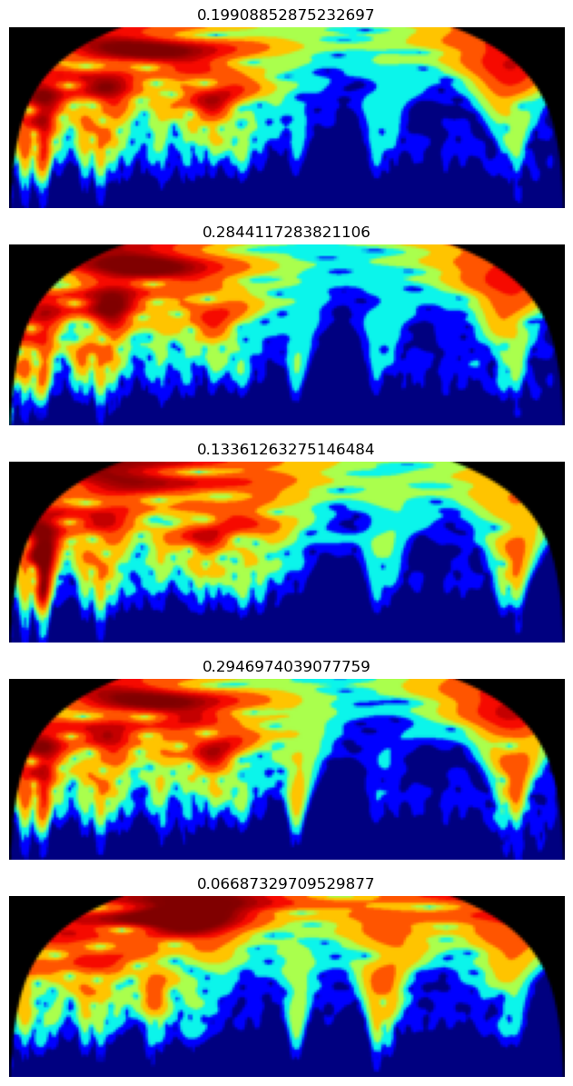

learn = vision_learner(dls, resnet18, pretrained=False, metrics=R2Score())

learn.lr_find()

SuggestedLRs(valley=0.00363078061491251)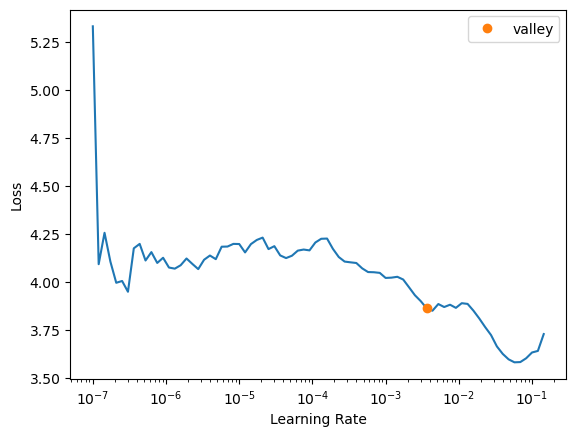

learn.fit_one_cycle(20, 2e-3)

epoch	train_loss	valid_loss	r2_score	time
0	1.010429	0.160208	-0.149856	07:33
1	0.101805	0.105252	0.244579	07:37
2	0.080996	0.092230	0.338037	07:45
3	0.061543	0.068272	0.509990	07:48
4	0.061344	0.045711	0.671919	07:57
5	0.055588	0.044312	0.681960	08:00
6	0.047412	0.038732	0.722007	08:06
7	0.042374	0.045522	0.673274	08:08
8	0.037796	0.034118	0.755128	08:07
9	0.030448	0.033509	0.759500	08:13
10	0.030273	0.034164	0.754792	08:07
11	0.025239	0.029398	0.788999	08:04
12	0.025301	0.028097	0.798343	08:02
13	0.022484	0.027496	0.802653	08:06
14	0.019801	0.025249	0.818778	08:07
15	0.016716	0.025171	0.819340	08:12
16	0.015120	0.024136	0.826770	08:10
17	0.012950	0.023746	0.829572	07:56
18	0.012212	0.024173	0.826501	07:47
19	0.012440	0.024042	0.827447	07:50

Evaluation

val_preds, val_targets = learn.get_preds(dl=dls.valid)

# Assuming you have a new CSV file for your test data
# test_source = '../../_data/ossl-tfm/ossl-tfm-test.csv'
# test_df = pd.read_csv(test_source)

# # Create a new DataLoader for the test data
# test_dl = learn.dls.test_dl(test_df)

# # Get predictions on the test set
# test_preds, test_targets = learn.get_preds(dl=test_dl)

# # Now you can use test_preds and test_targets for further analysis

# Convert predictions and targets to numpy arrays
# val_preds = val_preds.numpy().flatten()
# val_targets = val_targets.numpy()

# Create a DataFrame with the results
results_df = pd.DataFrame({
    'Predicted': val_preds,
    'Actual': val_targets
})

# Display the first few rows of the results
print(results_df.head())

# Calculate and print the R2 score
from sklearn.metrics import r2_score
r2 = r2_score(val_targets, val_preds)
print(f"R2 Score on validation set: {r2:.4f}")

   Predicted    Actual
0   0.153120  0.000000
1   0.189220  0.184960
2   0.325809  0.194201
3   0.442900  0.262364
4   0.335543  0.355799
R2 Score on validation set: 0.8270

val_preds_np = val_preds
val_targets_np = val_targets

# Apply the transformation: exp(y) - 1
val_preds_transformed = np.exp(val_preds_np) - 1
val_targets_transformed = np.exp(val_targets_np) - 1

# Create a DataFrame with the results
results_df = pd.DataFrame({
    'Predicted': val_preds_transformed,
    'Actual': val_targets_transformed
})

# Display the first few rows of the results
print(results_df.head())

# Calculate and print the R2 score
from sklearn.metrics import r2_score
r2 = r2_score(val_targets_transformed, val_preds_transformed)
print(f"R2 Score on validation set (after transformation): {r2:.4f}")

# Calculate and print the MAPE, handling zero values
def mean_absolute_percentage_error(y_true, y_pred):
    non_zero = (y_true != 0)
    return np.mean(np.abs((y_true[non_zero] - y_pred[non_zero]) / y_true[non_zero])) * 100

mape = mean_absolute_percentage_error(val_targets_transformed, val_preds_transformed)
print(f"Mean Absolute Percentage Error (MAPE) on validation set: {mape:.2f}%")

# Calculate and print the MAE as an alternative metric
from sklearn.metrics import mean_absolute_error
mae = mean_absolute_error(val_targets_transformed, val_preds_transformed)
print(f"Mean Absolute Error (MAE) on validation set: {mae:.4f}")

   Predicted   Actual
0   0.165464  0.00000
1   0.208306  0.20317
2   0.385151  0.21434
3   0.557217  0.30000
4   0.398699  0.42732
R2 Score on validation set (after transformation): 0.6978
Mean Absolute Percentage Error (MAPE) on validation set: 47.85%
Mean Absolute Error (MAE) on validation set: 0.1948

plt.figure(figsize=(6, 6))

# Use logarithmic bins for the colormap
h = plt.hexbin(val_targets, val_preds, gridsize=65, 
               bins='log', cmap='Spectral_r', mincnt=1,
               alpha=0.9)

# Get the actual min and max counts from the hexbin data
counts = h.get_array()
min_count = counts[counts > 0].min()  # Minimum non-zero count
max_count = counts.max()

# Create a logarithmic colorbar
cb = plt.colorbar(h, label='Count in bin', shrink=0.73)
tick_locations = np.logspace(np.log10(min_count), np.log10(max_count), 5)
cb.set_ticks(tick_locations)
cb.set_ticklabels([f'{int(x)}' for x in tick_locations])

# Add the diagonal line
min_val = min(val_targets.min(), val_preds.min())
max_val = max(val_targets.max(), val_preds.max())
plt.plot([min_val, max_val], [min_val, max_val], 'k--', lw=1)

# Set labels and title
plt.xlabel('Actual Values')
plt.ylabel('Predicted Values')
plt.title('Predicted vs Actual Values (Hexbin with Log Scale)')

# Add grid lines
plt.grid(True, linestyle='--', alpha=0.65)

# Set the same limits for both axes
plt.xlim(min_val, max_val)
plt.ylim(min_val, max_val)

# Make the plot square
plt.gca().set_aspect('equal', adjustable='box')

plt.tight_layout()
plt.show()

# Print the range of counts in the hexbins
print(f"Min non-zero count in hexbins: {min_count}")
print(f"Max count in hexbins: {max_count}")

Min non-zero count in hexbins: 1.0
Max count in hexbins: 180.0

path_model = Path('./models')
learn.export(path_model / '0.pkl')

Inference

ossl_source = Path('../../_data/ossl-tfm/img')
learn.predict(ossl_source / '0a0a0c647671fd3030cc13ba5432eb88.png')

((0.5229991674423218,), tensor([0.5230]), tensor([0.5230]))

df[df['fname'] == '0a0a0c647671fd3030cc13ba5432eb88.png']

	fname	kex
28867	0a0a0c647671fd3030cc13ba5432eb88.png	0.525379

np.exp(3) - 1

19.085536923187668

Experiments:

Color scale: viridis | Discretization: percentiles = [i for i in range(60, 100)]

Model	Image Size	Learning Rate	Epochs	R2 Score	Time per Epoch	Finetuning	with axis ticks
ResNet-18	100	1e-3	10	0.648	05:12	No	Yes
ResNet-18	224	2e-3	10	0.69	07:30	No	Yes
ResNet-18	750 (original size)	1e-3	10	0.71	36:00	No	Yes
ResNet-18	224	2e-3	20	0.704	07:30	No	Yes
ResNet-18	224	2e-3	10	0.71	07:00	No	No

Discretization: percentiles = [i for i in range(20, 100)]

Model	Image Size	Learning Rate	Epochs	R2 Score	Time per Epoch	Finetuning	with axis ticks	colour scale
ResNet-18	224	2e-3	10	0.7	05:12	No	No	viridis
ResNet-18	224	3e-3	10	0.71	05:12	No	No	jet

From now on with axis ticks is always No.

Discretization: esimated on 10000 cwt power percentiles [20, 30, 40, 50, 60, 70, 80, 90, 95, 97, 99]

Model	Image Size	Learning Rate	Epochs	R2 Score	Time per Epoch	Finetuning	remark	colour scale
ResNet-18	224	2e-3	10	0.71	05:12	No	None	jet
ResNet-18	224	2e-3	10	0.685	05:12	No	y range added	jet

From now on random splitter with 10% validation and random seed 41.

Discretization: esimated on 10000 cwt power percentiles [20, 30, 40, 50, 60, 70, 80, 90, 95, 97, 99]

Model	Image Size	Learning Rate	Epochs	R2 Score	Time per Epoch	Finetuning	remark	colour scale
ResNet-18	224	2e-3	10	0.7	05:12	No	Pre-train & normalize: True	jet
ResNet-18	224	2e-3	10	0.796	08:12	No	No Pre-train	jet
ResNet-18	224	3e-3	10	0.7	05:12	No	Pre-train & normalize: False	jet
ResNet-18 (id=0)	224	2e-3	20	0.829	08:12	No	No Pre-train (try 18 epochs)	jet