Visualization

Visualization tools for spectroscopic data.

The examples use the toy MIR dataset from load_toy_mir, and SNV from soilspectfm.preprocessing as an example transform:

from fastcore.test import *
from soilspectfm.preprocessing import SNV
from soilspectfm.datasets import load_toy_mir

deep_blue, blue, orange, red = '#0571b0', '#92c5de', '#f4a582', '#ca0020'

deep_blue, blue, orange and red are a diverging color palette for plots.

---

source

plot_spectra

def plot_spectra(
    X:numpy.ndarray, # Array of shape (n_samples, n_features) containing spectral data
    w:numpy.ndarray, # Array of wavelengths/wavenumbers corresponding to spectral features
    sample:int=50, # Number of spectra to randomly sample (if None, plot all spectra)
    ascending:bool=True, # Whether to plot wavelengths/wavenumbers in ascending order
    ax:matplotlib.axes._axes.Axes=None, # Optional matplotlib axes for plotting. If None, creates new figure
    **kwargs
)->matplotlib.axes._axes.Axes: # Additional parameters for plot customization

Plot spectra as lines against w

def plot_spectra(
    X: np.ndarray, # Array of shape (n_samples, n_features) containing spectral data
    w: np.ndarray, # Array of wavelengths/wavenumbers corresponding to spectral features
    sample: int = 50, # Number of spectra to randomly sample (if None, plot all spectra)
    ascending: bool = True, # Whether to plot wavelengths/wavenumbers in ascending order
    ax: plt.Axes = None, # Optional matplotlib axes for plotting. If None, creates new figure
    **kwargs # Additional parameters for plot customization
) -> plt.Axes:
    "Plot spectra as lines against `w`"
    def _prepare_data(X: np.ndarray, sample: int) -> np.ndarray:
        "Prepare data for plotting by sampling and reshaping if needed."
        if len(X.shape) == 1: return X.reshape(1, -1)
        if sample is not None: return X[np.random.choice(len(X), min(sample, len(X)), replace=False)]
        return X

    def _setup_axes(w: np.ndarray, ascending: bool, ax: plt.Axes, **params) -> plt.Axes:
        "Setup the axes with basic parameters."
        if ax is None: _, ax = plt.subplots(figsize=params.get('figsize', (20, 4)))
        
        _min, _max = np.min(w), np.max(w)
        _order = [_min, _max] if ascending else [_max, _min]
        ax.set_xlim(*_order)
        ax.grid(True, linestyle='--', alpha=0.7)
        ax.locator_params(axis="x", nbins=20)
        return ax

    def _set_labels(ax: plt.Axes, **params) -> None:
        "Set axes labels and title."
        ax.set_xlabel(params.get('xlabel', 'Wavenumber'))
        ax.set_ylabel(params.get('ylabel', 'Absorbance'))
        if params.get('title'): ax.set_title(params.get('title'))

    fig_params = dict(figsize=kwargs.pop('figsize', (20, 4)), xlabel=kwargs.pop('xlabel', 'Wavenumber'),
        ylabel=kwargs.pop('ylabel', 'Absorbance'), title=kwargs.pop('title', None))

    line_params = dict(alpha=0.6, color='#333', lw=1) | kwargs

    X = _prepare_data(X, sample)
    ax = _setup_axes(w, ascending, ax, **fig_params)
    
    for spectrum in X: ax.plot(w, spectrum, **line_params)
    
    _set_labels(ax, **fig_params)
    
    return ax

plot_spectra draws each spectrum as a line against w. It plots sample spectra picked at random without repeats, or all of them when sample is None or exceeds the number of spectra. It creates a new figure, or draws on ax when you pass one, and returns the axes. figsize, xlabel, ylabel and title set the figure, and other keyword arguments go to ax.plot. The toy dataset has 50 spectra, so the default sample=50 draws each of them once:

X, ws = load_toy_mir()
ax = plot_spectra(X, ws, ascending=False, alpha=0.5)
test_eq(len(ax.lines), 50)
test_eq(len({line.get_ydata().tobytes() for line in ax.lines}), 50)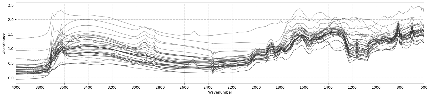

Passing ax puts several plots in one figure. The returned axes accept further matplotlib customization, such as axis limits. Here, raw and SNV-corrected spectra share one figure:

fig, (ax1, ax2) = plt.subplots(2, 1, figsize=(15, 7))
ax1 = plot_spectra(X, ws, ax=ax1, ascending=False, color='black', alpha=0.4, lw=0.5, xlabel='Wavenumber (cm$^{-1}$)', title='Raw Spectra')
ax2 = plot_spectra(SNV().fit_transform(X), ws, ax=ax2, ascending=False, color=deep_blue, alpha=0.4, lw=0.5,
    xlabel='Wavenumber (cm$^{-1}$)', title='Preprocessed (SNV) Spectra')
ax1.set_ylim(0, 2.5)
ax2.set_ylim(-2.5, 2.5)
plt.tight_layout()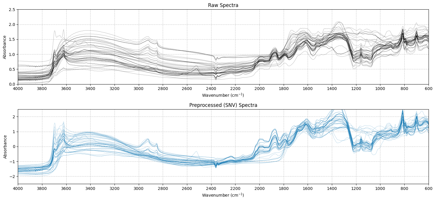

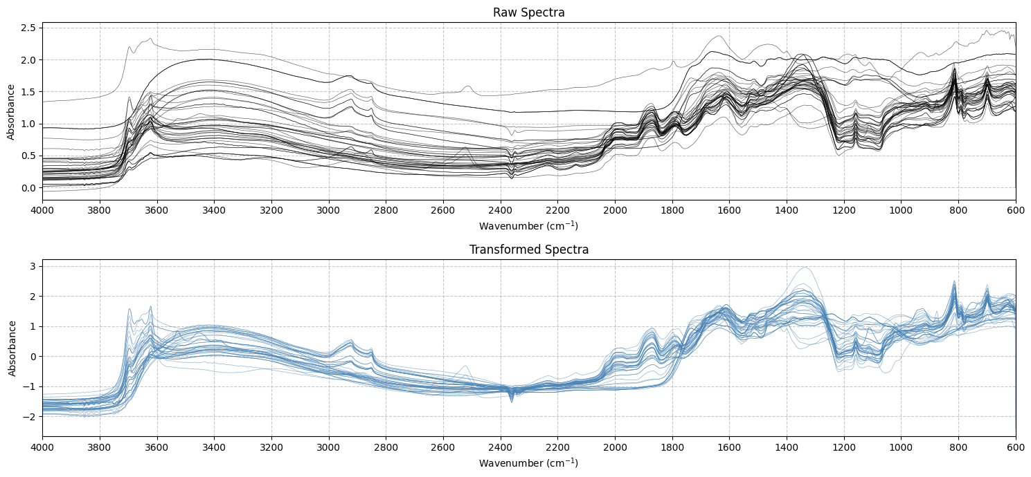
plot_spectra_comparison draws that two-panel figure in one call, with raw spectra above and transformed spectra below. It returns the figure and both axes:

---

source

plot_spectra_comparison

def plot_spectra_comparison(
    X_raw:numpy.ndarray, # Raw spectra, shape (n_samples, n_features)
    X_transformed:numpy.ndarray, # Transformed spectra, same shape as `X_raw`
    wavenumbers:numpy.ndarray, # x-axis values for both panels
    raw_title:str='Raw Spectra', # Title of the upper panel
    transformed_title:str='Transformed Spectra', # Title of the lower panel
    figsize:tuple=(15, 7), # Figure size
    **kwargs
):

Plot raw and transformed spectra in two panels, one above the other

def plot_spectra_comparison(
    X_raw: np.ndarray, # Raw spectra, shape (n_samples, n_features)
    X_transformed: np.ndarray, # Transformed spectra, same shape as `X_raw`
    wavenumbers: np.ndarray, # x-axis values for both panels
    raw_title: str='Raw Spectra', # Title of the upper panel
    transformed_title: str='Transformed Spectra', # Title of the lower panel
    figsize: tuple=(15, 7), # Figure size
    **kwargs # `raw_color`, `transformed_color`, and other arguments for `plot_spectra`
):
    "Plot raw and transformed spectra in two panels, one above the other"
    raw_color = kwargs.pop('raw_color', 'black')
    transformed_color = kwargs.pop('transformed_color', 'steelblue')
    fig, (ax1, ax2) = plt.subplots(2, 1, figsize=figsize)
    common_params = dict(ascending=False, alpha=kwargs.pop('alpha', 0.6), lw=kwargs.pop('lw', 0.5), xlabel='Wavenumber (cm$^{-1}$)') | kwargs
    ax1 = plot_spectra(X_raw, wavenumbers, ax=ax1, color=raw_color, title=raw_title, **common_params)
    ax2 = plot_spectra(X_transformed, wavenumbers, ax=ax2, color=transformed_color, title=transformed_title, **common_params)
    plt.tight_layout()
    return fig, (ax1, ax2)

plot_spectra_comparison(X, SNV().fit_transform(X), ws, raw_title='Raw Spectra', transformed_title='Transformed Spectra');